IRIS Dataset Classification using KERAS library

Supervised Learning

Data points have known labelled outcome.

Goal is to predct the nature of relationship between input parameters and target variables.

Parameters: of a machine learning model are 1 or more variables that changes their values as the model learns. No of parameters can range from very few to trillions of parameters.

Hyperparameters: are parameters that not learned directly from the data but relates to implementation.

Two types of problems:

Regression: y or the outcome variable is numeric.
- Outcome is continuous.
Classification: y or outcome variable is categorical.
- Outcome is categorical.

Some terms of interests are:

x: input features
yp: Output or the predicted values
f(.): prediction function that generates predictions from x and parameters.
J(y,yp): Loss function
update rule: using features x and outcome y, choose parameters to minimize loss function J

Interpretation vs Prediction Objective:

Interpretation: Train model to find insights into data. Focus will be on parameters of the model to gain insights; and a less complex models are chosen.
Prediction: focus will be on performance metrics of the model. The model cares only about coming with best prediction so can be a black box; complex models can be used. performance metrics involve closeness between yp and y i.e. predicted result vs actual result.

Linear Regression

Measures of errors are: They can be used for any regression model

Mean Squared Error (MSE)
Sum of Squared Error (SSE) = sum (error^2)
Total Sum of Squares (TSS) = Variance of error
Coeffecient of Determination (R^2): 1-(SSE/TSE). Closer to 1 is better.

It is not a requirement that the target variable is normally distributed; but normally distributed target variable gives better result. What is required is that the error needs to be normally distributed.

If the target variable is not normally distributed, you can make it by transforming it. Then, fit our regression to the transformed values.

To see if the target variable is normally distributed, we can see manually or do a statistical test.

For manual approach, we can plot the distribution using df['target_variable'].hist() . It should visually show the data thus helping us see if the data is normally distributed.
Using D'Agostino K^2 Test , you can use library function normaltest() from library scipy.stats.mstats . This gives out a p-value. The higher p-value indicates the distribution is more closer to being normal. A lower p-value indicates distribution is far low probability of being a normal distribution. A threshold of 0.05 or 0.01 can be used for cutoff.

To transform a variable (target variable) to make it normally distributed, commonly used techniques are:

Log transform: Just take log of the data. The data will look a lot more normal distributed. This works best for data that exhibits exponential property.
Square Root: Just take square root of the data.
Box Cox: It is a parameterized transformation.
- Box-Cox transformed value of a variable y is (y^lambda -1)/lambda.
- This is a generalization of the square root transformation, but it allows for the root value to vary and find the best one.
- Use boxcox from scipy.stats in code; as y_transformed = boxcox(df['y'])[0] . Function boxcox returns an array, the first item is the transfored array whereas the second item the lambda that was used.

How to use:

Import sklearn library as sklearn.linear_model.LinearRegression
create an object as LR=LinearRegression() . You can also pass many other hyperparameters into the object creation.
Create X df from the actual dataset by dropping the target variable column so that it is easy for further computation. Similarly, create Y by just grabbing the target variable as it column.
Fit and transform the X data with the polynomial feature object.
- First create an object as pf = PolynomialFeature(degree=2,include_bias=False) , that is from sklearn.preprocessing . The include_bias is False because later on LinearRegression will take care of that part.
- Fit and transform as X_pf = pf.fit_transform(X) . X_pf now has a lot more columns that what X had.
Test-Train split:
- x_train, x_test, y_train, y_test = test_train_split(X_pf,y,test_size=0.3,random_state="some int value") where test_train_split is from sklearn.model_selection .
Now apply standard scaler to the train data.
- s = StandardScalar()
- x_train_s = s.fit_transform(x_train)
Now to bring the target variable to the normal distribution, we will use boxcox as discussed above.
- y_train_bc = boxcox(y_train)[0]
- We also need the lambda value for later when we need to compute inverse. so, lam=boxcox(y_train)[1]
Fit the train data as LR = LR.fit(x_train_s, y_train_bc) . Here we used:
- standard scalar fit and transfored x- data.
- boxcoxed y- data
Since the x- data used for modeling was transformed data, let us fit and transform the x_test data to StandardScalar, i.e. x_test_s = s.transform(x_test)
The predicted value will be boxcoxed transformed; i.e. y_pred_bc = lr.predict(x_test_s) .
To find the y_pred_bc back to the same scale as y, we can inverse boxcox. y_pred = inv_boxcox(y_pred_bc,lam) .
Finally, compute the R2 score using R2 = r2_score(y_pred,y_test) .
Using boxcox on the target variable improves the R2 score (higher is better). In the above example, if done without boxcox, the R2 score will be lower.

Data Splits and Cross Validation

To split to have a hold out data, so that its used for cross validation.

Training data:

Used for training.
model(x_train,y_train).fit() = model

Test data:

Used for testing and prediction.
model.predict(x_test) = y_pred

Use actual y_test to compare and calculate test_error .

Syntax for test train split

from sklearn.model_selection import test_train_split
train,test = test_train_split(data,test_size=0.3)
x_train,x_test, y_train, y_test = test_train_split(x,y,test_size=0.3)
There are other many ways for splitting, like shuffle split or stratified shuffle split.
from sklearn.model_selection import ShuffleSplit

Categorical Data is one-hot encoded. The number of columns that is made as a result of one-hot encoding is equal to no of category values - 1. The process is outline below:

Find the columns whose dtypes is np.object, i.e. mask = df.dtypes==np.object .
And, filter out the columns cols = df.columns[mask] . These are the columns that we want to apply one-hot encoding to.
We would also like to see if the no of unique values in the columns are more than one. If there is only 1 unique value, it does not make sense to one-hot encode.

Using sklearn.preprocessing.OneHotEncoder , instead of pd.get_dummies

df_copy = df.copy()
instantiate one hot encoder object, ohc = OneHotEncoder()
inside a for loop for each column, col in the cols list:
- dat = ohc.fit_transform(df_copy[col])
- drop the original column, df_copy.drop(col,axis=1)
- get the name of all the new columns, new_cols = ohc.categories_
- create name of columns so that its easy to join in the df later
  new_cols = ['_'.join([col,catt]) for cat in new_cols[0]]
- create a df from the one hot encoded data
  new_df = pd.DataFrame(dat.toarray(),columns=new_cols)
- now append to our copy df
  df_copy = pd.concat([df_copy,new_df],axis=1 )
One potential issue with too many one-hot encoded df is that Too many parameters, overfitting of model. Error will be high in test data is overfit.

Another way of dealing with categorical data is using LabelEncoder class in sklearn. This encoder should be used for encoding the target value, y, not the input variables X. It transforms the columns into numerical values from 0 to (num. of unique values -1).

from sklearn.preprocessing import LabelEncoder

le = LabelEncoder
df['col1'] = le.fit_transform(df['col1'])

Applying scalar like StandardScalar or MinMaxScalar , make sure to call fit_transform() on the training data; but only transform() on the test data. This should be done before applying linearregression. An example is given below.

create an object, for example
s = StandardScalar()
fit transform x_train data
x_train_s = s.fit_transform(x_train)
transform x_test data
x_test_s = s.transform(x_test)
fit the linearRegression model
LR.fit(x_train_s,y_train)
predict
predictions = LR.predict(x_test_s)
find error
error = mean_squared_error(y_test,predictions)

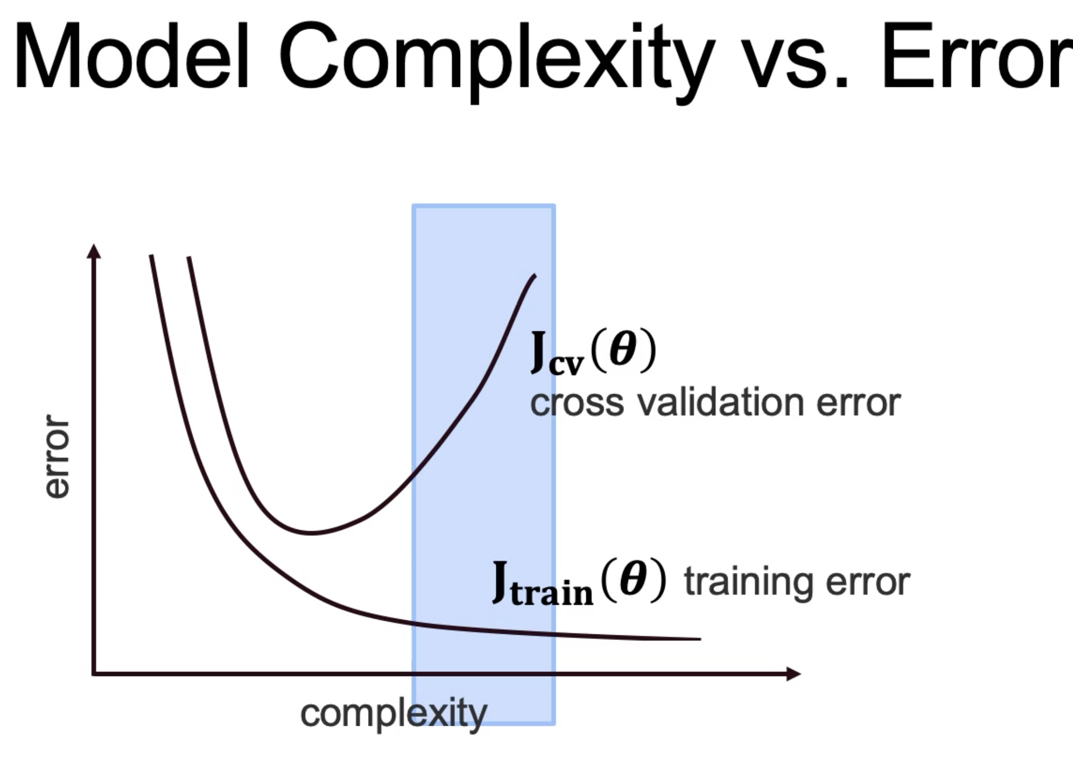
Cross Validation

Here we use multitple validation sets. These are test sets that are disjoint of each other. For each case of validation sets, the train dataset can be a subset of the remaining dataset. There should be no overlap between the validation or test splits in each iteration of experiment. Training data can have overlap.

The average error across all these validation sets is the cross validation result .

As the model gets more complex, the train error will minimize. But with the cross validation, there is an inflection point, and as the complexity increases, the error will increase. This is because too complex model will not generalize properly, and overfit. This we should stop increasing the complexity as soon as the crossvalidation error starts to increase.

Coding example:

import library
from sklearn.model_selection import cross_val_score
perform cross val score
cross_val = cross_val_score(model, x_data, y_data, cv=4, scoring='neg_mean_squared_error')
Other methods as follows are also available from sklearn.model_selection import KFold, StratifiedKFold

Using Pipeline and Crossvalidation

Import all needed library from sklearn.linear_model import LinearRegression, Lasso, Ridge
From the dataset, acquire the target variable as Y, and drop the value from original df to save it as X.
Use kfold that is imported as
from sklearn.model_selection import KFold, cross_val_predict
kf = KFold(shuffle=True, random_state=6644, n_splits=3)
This means we will have 3 training and 3 test sets. Training sets may overlap, but test sets will not overlap.
kf.slit(X) will give a generator object that has indices. For example, iterating through the generator gives a tuple with x-indices and y-indices as follows:
for train_index, test_index in kf.split(X):
The index values, train_index, test_index can be anything from 0 to length of X-1, with length being determined by the split value.
Once the indices are obtained, extract the value from the X and Y using the indices.
for train_index, test_index in kf.split(X):
..X_train,X_test, y_train, y_test = (X.iloc[train_index], X.iloc[test_index],y[train_index],y[test_index])
..lr.fit(X_train, y_train)
..y_pred = lr.predict(X_test)
..score = r2_score(y_test.values, y_pred)

This will show the scores for all the splits.
Let us add standard scalar into this. Without any regularization, scaling does not help Linear Regression. But just to see an example, following can be done.
s = StandardScalar()
for train_index, test_index in kf.split(X):
..X_train,X_test, y_train, y_test = (X.iloc[train_index], X.iloc[test_index],y[train_index],y[test_index])
..X_train_s = s.fit_transform(X_train)
..lr.fit(X_train_s, y_train)
..X_test_s = s.transform(X_test) ..y_pred = lr.predict(X_test_s)
..score = r2_score(y_test.values, y_pred)

This will show the scores for all the splits.

Using pipeline

Sklearn allows to chain multiple operator items, as long as as they have fit() method.
Here, output of one is input of another. So they also need to have fit_transform() method.
The above code will now be following using pipeline:
- s = StandardScalar()
  lr = LinearRegression()
- my_pipe = Pipeline([('scalar',s),('regression',lr)])
- kf = KFold(shuffle=True, random_state=6644, n_splits=3)
- predictions = cross_val_predict(my_pipe,X,y,cv=kf)
- r2_score(y,predictions

HyperParameter Tuning, Lasso Regression, PolynomialFeature

function used is np.geomspace
For Lasso Regression , higher value of alpha means the model is less complex whereas lower value of alpha means model is more complex.
Less value of alpha for lasso makes the model similar to LinearRegression.
Lasso is iniitalized as
lasso=Lasso(alpha=alpha, max_iter=10000)
Complete usage with different values of alpha for hyperparameters selection is as follows:
alphas = np.geomspace(1e-9,1e10,num=10) #creates equally spaced 10 numbers, geometrically spaced
for alpha in alphas:
.. lasso = Lasso(alpha=alpha,max_iter=100000)
.. my_pipe = Pipeline([('scalar':s),("lasso":lasso)])
.. pred = cross_val_predict(my_pipe,X,y,cv=kf)
.. score = r2_score(y,pred)
With Lasso, its is always better to scale the data before using lasso regression.

You can add PolynomialFeature to the pipeline. What a PolynomialFeature does is very well explained at this link . In a nutshell, it raises the input variables to a polynomial degree. So, after applying the PolynomialFeature, the input dimension now increases.

The above example thus becomes:

pf = PolynomialFeature(degree=3)
alphas = np.geomspace(1e-9,1e10,num=10) #creates equally spaced 10 numbers, geometrically spaced
for alpha in alphas:
.. lasso = Lasso(alpha=alpha,max_iter=100000)
.. my_pipe = Pipeline([('polyfeat':pf),('scalar':s),("lasso":lasso)])
.. pred = cross_val_predict(my_pipe,X,y,cv=kf)
.. score = r2_score(y,pred)

After going through the different scores based on various alpha values, we can find the best among all. And finally train the model as follows:

best_pipe = Pipeline([
("poly_feat":PolynomialFeature(degree=2)),
("scalar":s),
("lasso":Lasso(alpha=0.01,max_iter=100000))
])
best_pipe.fit(X,y)
best_pipe.score(X,y)
To see the coeffecients, we can
best_pipe.named_steps['Lasso'].coef_
Ridge Regression also works the same way as far as the coding aspect is concerned.
From the pipeline estimator that we created, we can actually see the interaction of the different input variables and the their contribution to the output variable.

From the pipeline, polynomial feature gives the higher power of the input variable as well as the interaction components. The corresponding coefficient of the Lasso/Ridge regression model will indicate their relative contribution. Higher positive value indicates positive impact whereas higher negative value indicates negative impact.

from the best_pipe.named_steps['poly_feat'].get_feature_names(input_features=X.columns) gives the feature names whereas as seen before .coef_ gives the lasso/ridge coefficient.

Stratified cross validation is not equivalent to k-fold cross validation with k=N-1 where N is no of features.

For a linear regression model, stratified cross-validation with same k will not increase the variance of estimated parameters, as compared to k-fold cross validation.

For k-fold cross validation, variance of the estimated model parameters will increase across subsamples with increase in k.

Grid Search CV

define pipeline as follows
estimator = Pipeline ([
.. ('polynomial_features', PolynomialFeatures()),
.. ('scalar',StandardScalar()),
.. ('ridge_regression',Ridge())
.. ])
create parameters as following:
params = {
'polynomial_features__degree' : [1,2,3],
'ridge_regression__alpha' : np.geomspace(4,20,30)
}
The name of the items keys in parameters dict comes from PipeLine component name + two underscores + its property
create a GridSearchCV() object as:
grid = GridSearchCV(estimator, params,cv=kf)
Fit the data:
grid.fit()
Predict as
y_predict = grid.predict(X)
Print the best metrics as
grid.best_score_, grid.best_params_
If we want to look at the coeff of the estimators, we can do following
grid.best_estimator_.named_steps['ridge_regression'].coeff_
To see the scores for all the variables that it searched through, and the scores obtained for each of those variables
pd.DataFrame(grid.cv_results_)

polynomial Regression

Following are some of the approaches for dealing with fundamental problems of prediction and interpretation :

Extending linear regression
using polynomial features to capture non-linear effects.

We want to capture higher order features of data by adding polynomial features. The relation may still be linear, but with a higher degree terms.

This can also include variable interactions,like x1x2 in addition to x1^2 and x2^2 from x1 and x2.

Using polynomial features example as somewhere above, we do following:

create polyFit with degree of m
fit the X data
transform the X data

This will create the interaction terms also.

Bias and Variance

Bias : is a tendency to miss. They are guided by similar error, and are generally with low variance and the data points are consistently errored.

Variance : is a tendency to be inconsistent. It can be thought of as a metric to refer to model's sensitivity.

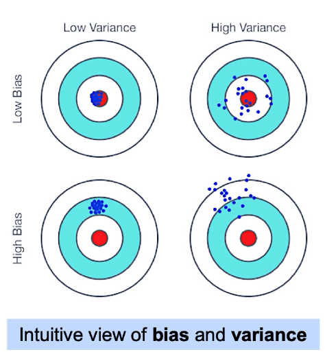
Above image shows an example for definition of Bias and Variance in terms of shooting to an target. Ideally, we would want our model to have an outcome that is top-left outcome , with small bias and the preditions (or shootings) very close to the target.

Three Source of Errors in a Model :

Model being wrong: Bias
- Can be because of missing information
- Can be because of simple model
- Miss real pattern, because model is underfit.
Model being unstable: Variance
- Characterized by high changes in the output because of small changes in the input.
- Overly complex or poorly fit models
- Overfitting of model
Unavoidable Randomness: Random error that cannot be reduced

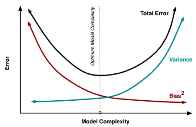
For polynomial regression, higher degree means model is complex. Thus high variance and lowered bias.

Regularization and Model Selection

Regularization is an approach to handle over-fitting.

Add a new cost function to the old cost function, with a Regularization Strength Parameter . Thus a new cost adjusted cost function is created as M(w) + lambda * R(w) , where M(w) is the model error, R(w) is the function of estimated paramters and lambda is the strength parameter.

The adjustable regularization strength paramter can be used to penalize the model if it is too complex. This can be used to dumb down the model. lambda adds a penalty propoortional to the size of the estimated model parameter.

Regularization strength parameter allows us to manage complexity tradeoffs:

more regularization, less complex model or more bias
less regularization, more complex model or increased variance

L1 Regularization: Drives some coeffecients dowm to zero, because the added model parameters values are single degree multiplied by the lambda.
L1 regularization imposes Laplacian prior.
L2 Regularization: On the other hand, adds squared model parameters to the cost function.
L2 regularization imposes Gaussian prior.

Ridge Regression

Ridge Regression is a L2 regularized linear regression.
There is influence of standardization on Ridge regression.
Regularization has shrinking effect, some coeffecients towards 0 due to the penalty. The added term is the difference between the Linear Regressio and Ridge Regression. It uses L2 regularization on linear regression.
There is squaring, so larger weights are more penalized.
As regularization strenght increases for ridge regression, the shinkage effect is seen, i.e., we will decrease each coeffecients.
The reduction of variance may outpace the increase in bias, which leads to better model.
With ridge regression, we have RidgeCV , that also perform cross validation at the same time.
from sklearn.linear_model import RidgeCV
alphas = [0.005, 0.01, 0.05, 0.1]
ridcv = RidgeCV(alpha=alphas,cv=4).fit(x_train, y_train)
v_pred = ridcv.predict(x_test)
The best alpha value can be extracted as ridcv.aplha_ , and the coeffecients of the model can be listed as a list ridcv.coef_

Lasso Regression

Lasso is L1 regularized Linear Regression. LASSO stands for Least Absolute Shrinkage and Selection Operator
The complexity penalty lambda is proportional to the absolute value of the coeffecients.
More likely to perform feature selection , because it will zero out some of the terms as it uses L1 regularization.
Lasso have higher interpretability than Ridge. But is slower to converge than Ridge so the timing may be high for Lasso.
May also underperform if the target truly depends on many of the features.
We also have a lassocv similar to Ridge cv discussed above. An additional term to provide is nax_iter because lasso does not converge as fast.

Elastic Net

A hybrid approach that introduces a new parameter alpha that determines a weighted average of L1 and L2 penalties.
ElasticNetCV is also a class similar to LassoCV and RidgeCN, but with an additional parameter called l1_ratio in addition to l1_ratio and alphas.

Recursive Feature Elimination (RFE): RFE is an approach that combines

a model or estimation approach;
a desired number of features

RFE repeatedly applies the model, measures feature importance and recursively removes the less important features.

RFE example is as follows:
from sklearn.feature_selection import RFE
rfe = RFE(est, n_features_to_select=5)
rfe = rfe.fit(X_train, y_train)
y_pred = rfe.predict(X_test)

A class RFECV , uses RFE with cross validation.

regularization forces the range of coefficients to be smaller, restricted. Smaller range of coeffecients will have lower variance.

So overall steps as of now for LinearRegression are:

Isolate target variable as y.
y = df[y_col]
Create other cols as X
X = df.drop[y_col,axis=1]
test train split
Apply standardization to the data. Most common is to use StandardScalar .
s = StandardScalar()
X_s = S.fit(X)
Apply LinearRegression
lr = LinearRegression()
lr = lr.fit(X_s, y)
See the coeffecients
print(lr.coef_)
To see what input vairable has what coeff, we can do following:
pd.DataFrame(zip(X.columns,lr2.coef_)).sort_values(by=1)

For Lasso Regression, we introduce the PolynomialFeatures with certain degree also.

First, fit_transform() with PolynomialFeature
test train split
Then, fit_transform(x_train) with StandardScalar
Then, lasso().fit(x_train,y)
Then lasso().predict(StandardScalar.transform(x_test))
Then, compute r2_score or something

Logistic Regression

Used for classification. An extension of Linear Regression but handles what Linear Regression gets wrong.

Sigmoid Function

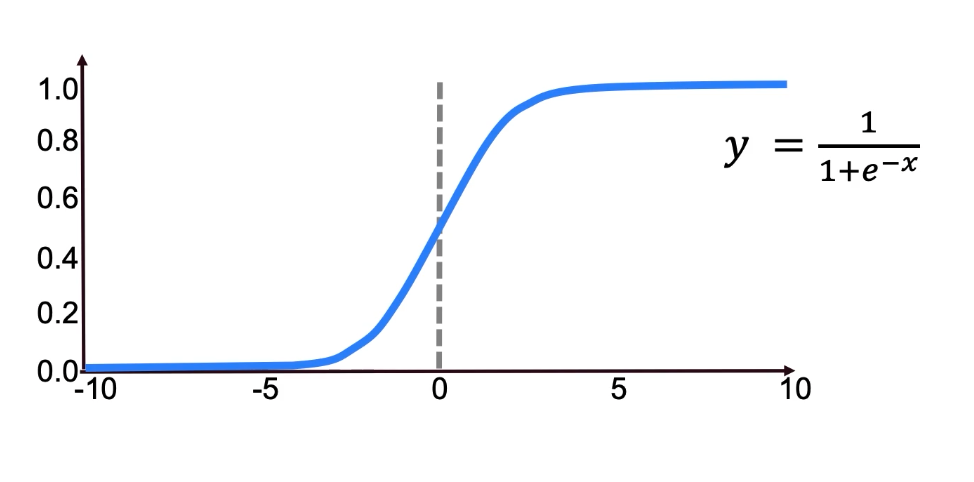
The use of sigmoid can be useful for classification in some of the obvious separable classes (for example), as below image prsents.

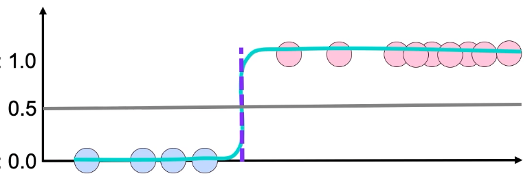
We can see how it can classify between two classes with a clear decision boundary.

import sklearn.linear_model import LogisticRegression
lr = LogisticRegression(penalty='l2', c=10.0)
lr = lr.fit(x_train, y_train)
y_predict = lr.predict(x_test)
lr.coef_
Above, c is the regularization constant (here higher c means less lambda, so is inverse).

LogisticRegression also comes with LogisticRegressionCV.

Confusion Matrix :

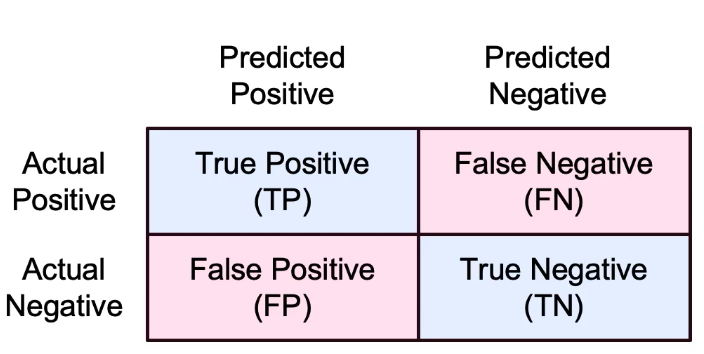
False Positive: Type-I error
False Negative: Type-II error
Accuracy = (True Positive + True Negative)/All Observations
- Correct predictions divided by total no of predictions.
- Is most useful when the classes are balanced, i.e., when the no of items in both the correct and incorrect classes are similar.
- Not a good choice for unbalanced situations.
Recall/Sensitivity = (True Positive)/(True Positive + False Negative)
- Ability of a model to find all the relevant cases within a dataset..
- But a major flaw here is a model can predict all as True Positive, and have a 100% Recall.
Precision = (True Positive)/(True Positive + False Positive)
- Ability of a model to find ONLY the relevant cases within a dataset.
- It quantifies what portion of the datapoint that the model found relevent were actually relevant.
- Precision helps to balance the flaw of Recall. It shows how often, from among the positive predicted values, it gets the prediction correct.
Specificity = (True Negative)/(False Positive + True Negative)
Specificity is the recall for negative class.
F1 Score = Harmonic Mean of Precision and Recall = 2* (Precision * Recall)/(Precision + Recall)
- This is the optimal blend of both the precision and recall.
- Harmonic Mean is taken instead of simple average because harmonic mean will punish the extreme values. For example, in case where one is 0 and other is 1, simple average is 0.5 which does not really reveal the extremety of the value. But HM is 0, which shows one of the values is 0.

ROC Curve: Receiver Operating Characteristic

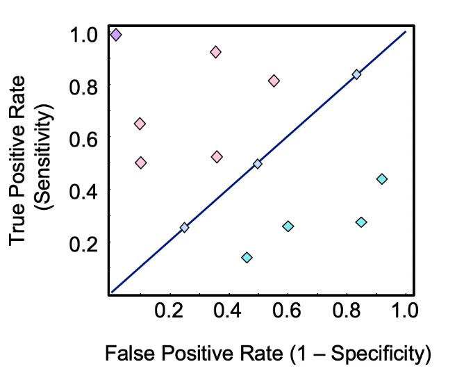
Curve of True Positive Rate vs False Positive Rate . False Positive Rate is computed as 1-Specificity .
The diagonal line is random guess.
Lower than diagonal is worse .
Higher than diagonal is good .
This is because True Positive needs to be relatively higher than False Positive Rate.
Area use the curve of the ROC curve gives how well the mode is working. Higher is better.

What is the right approach for choosing the classifier:

ROC curve: works better with balanced classes.
Precision-Recall works better with imbalanced classes.

In sklearn
from sklearn.metrics import accuracy_score
accuracy_value = accuracy_score(y_test,y_pred)

Other accuracy metrics,
from sklearn.metrics import precision_score, recall_score, f1_score, roc_auc_score, confusion_matrix, roc_curve, precision_recall_curve

Logistic regression example

if the output variable is categorical, which it usually is for logistic regression problem, let us convert to numerical using LabelEncoder
let us also look into the correlation between the input or independent variables. This can be done by
corr = df[array of columns].corr() that returns a dataframe
since the lower traingle of the corr() does not give any new information, we can set them as null by following technique.

#gets the indices as 2D numpy array, x in first dim and y in second dim corr_low_index = np.tril_indices_from(corr) #convert the df above to numpy array corr_np = np.array(corr) #set the low diagonal elements to nan corr_np[corr_low_index] = np.nan #convert back to the df corr_df = pd.DataFrame(corr_np,columns=corr.columns,index=corr.index) corr_df_stack = (corr_df.stack() .to_frame().reset_index() .rename(columns={'level_0':'feature1', 'level_1':'feature2', 0:'correlation'} ) ) #let us stack the df for a more compact df corr_df_stack['abscorrelation'] = corr_df_stack.correlation.abs()
The above final db can help us see what values are highly correlated, if we sort them by the absolute value column
To maintain the ration of the predictor class in the train and test splits, we can use StratifiedShuffleSplit class.

from sklearn.model_selection import StratifiedShuffleSplit # We want 1 split, this can change if we want more # .. 30% data to be in the test dataset, 70% in train dataset my_split = StratifiedShuffleSplit(n_splits=1, test_size=0.3, random_state=23345) train_idx, test_idx = next(my_split.split(data[x_colms], data.target)) X_train = data.loc[train_idx, x_colms] y_train = data.loc[train_idx, 'target'] X_test = data.loc[test_idx, x_colms] y_test = data.loc[test_idx, 'target']

k-Nearest Neighbour Classification

We can also do regression using kNN; the value predicted is the mean value of its neighbors.

creates decision boundary based on similarity with neighbors whose class is already known.
using small number of neighbors to look at may be prone to high error.
increasing the number of neighbors to look at will decrease the error.
using a very high number of neighbors also causes error to go up. So, there is an elbow point for the minimum error rate.
using one- neighbor for classification will cause highly biased system
using more neighbor than the elbow point causes high variance

Distance measurement in kNN:

Euclidian Distance: Visible distance., the easiest distance.
Manhattan Distance: Absolute value in each direction. Unlike Euclidian, there is no squaring and taking a square root here.
Oftentimes scaling the features is a good strategy, so that all the variables have same influence.

Easy to use;
Adapts well to new training data;
Easy to interpret
cons: no model for insights;
cons: slow to predict, many distance calculations;
cons: require a lot of memory;
cons: may break down because of curse of dimensionality as the number of predictors grow

kNN is faster for fitting, as only trainig data storing is sufficient. LinearRegression fitting can be slow.
kNN is many parameters; Linear Regression has new parameters, so memory efficient than kNN.
kNN prediction can slow; Linear Regression prediction involves calculation but are often fast.

from sklearn.neighbors import KNeighborsClassifier kNN = KNeighborsClassifier(n_neighbors=3) kNN = kNN.fit(X_train, y_train) y_predict = kNN.predict(X_test)

For regression, KNeighborsRegressor can be used instead, and make sure that the y_train and y_test sets are continuous values.

Support Vector Machines (SVM)

create a hyperplane that maximizes the distance between the nearest member of all the classes;
the cost function does not penalize for output that are outside the margin if the prediction is correct; whereas in case of logistic regression there is almost always some penalization.
If the values are classified correctly, and are inside the margin lines, it adds to the penalty, i.e. model is penalized.
The more we move to the opposite direction for misclassification, model is penalized more. The penalty value is linearly increased.
The SVM model could be sensitive to outliers, and the decision boundary may shift significnatly because of a single outlier. Thus, regularization . However, SVM is not impacted by large values that are classified correctly. Or any outlier that are correctly classified.
SVM models are linear (decision boundary is linear hyperplane).
Code example:
from sklearn.svm import LinearSVC LinSVC = LinearSVC(penalty='l2',C=10.0) #C is regularization LinSVC = LinSVC.fit(X_train,y_train) y_pred = LinSVC.predict(X_test)
The regilarization parameters can be explored/tuned with cross-validation.
Using linearSVM for regression; and y- values must be continuous values.
from sklearn.svm import LinearSVM

Non Linear Decision boundaries using kernels.

Just change the objective function; non-linear decision boundary is created by tranforming the variables and finding the linear decision boundary in the new variables; which essentially means that the decision boundary is now non-linear in original vector space.
Map data to higher dimension. As we move above in dimensionality, there could be some linear decision boundary that could be found.
- Approach 1: Similar to polynomial transform.
- Approach 2: FInd similarity metric/function, and use that function to transform to higher dimension.
  - Create a Gaussian distance function.
  - Find similarity of the variables to the n- variables that the Gaussian distance is defined for. The new vector space will be n-dimensional, with each dimension representing similarity to the n- variables.
Code example:
from sklearn.svm import SVC rbfsvc = SVC(kernel='rbf', gamma=1.0, C=10.0) # see other kernels, higher gamma and C means less regularization/complex models. rbfsvc = rbfsvc.fit((X_train, y_train)) y_predict = rbfsvc.predict(X_test)
Kernels with rbf are very slow to train with a lots of features of data.
To optimize, use a kernel map to create a dataset in higher dimension using methods like Nystroem and RBF sampler. Then, use a linear classifier, like LinearSVC, or even LogisticRegression.
Nystroem example:
from sklearn.kernel_approximation import Nystroem NystroemSVC = Nystroem(kernel='rbf', gamma=1.0,n_components=100) # n_components means the no of samples to take X_train = NystroemSVC.fit_transform(X_train) X_test = NystroemSVC.transform(X_test)
The kernel and associated parameters can be tuned with cross-validation
Similar can be done for RBFSampler

When to choose what??

Features	Data	Model
Many (~10K)	Small (1K rows)	Simple, Logistic or Linear SVC
Few, near about 100	Medium (~10K rows)	SBC with RBF
Few, near about 100	Many (>100K rows)	Add features, Logistic, LinearSVC or Kernel Approx

Decision Trees

Keep splitting until a leaf node is pure OR a max depth is reached OR a performance metric is achieved.
Decision trees tend to overfit. Small change in data greatly affect prediction - high variance.
Solution: Prune Trees by imposing max depth
Pruning can be done by applying error threshold. (for example, if the error at a node is X, dont further breakdown)
Very easy to interpret, no data processing required

Regression can be performed using DecisionTreeRegressor ,where the target variable is a continuous field.

Ensemble Methods and Bagging (MetaClassifiers)

Bootstrap Aggregation is Bagging.
Combining models (ensemble based methods)
For example; for decision trees that tend to overfit, we can create many trees and combine results.
- So we use bagging for trees using BaggingClassifier .
- trees vote or average of the predicted result or take majority as a result
- i.e. vote to combine to form a single classifier.
- No of trees to use for Bagging is another hyperparameters. There is a diminishing return usually after 50 trees.
- Bagging Trees is again easy to interpret and implement. No preprocessing required.
- Bagging, we can grow trees parallely and is more efficient.
from sklearn.ensemble import BaggingClassifier BC = BaggingClassifier(n_estimators=50) #n_estimators is the no of trees BC = BC.fit(X_train, y_train) y_pedict = BC.predict(X_test)
For regression, BaggingRegressor can be used.

Random Forest

Bootstrapped samples can be correlated, so bagging may not always work after some number.
To de-correlate the trees, we use a random subset of features of each tree.
so we limit the total no of features used randomly; in addition to randomly limiting the rows which is already done by Bagging.
For classification, we restrict the features to sqrt(no of features) , whereas regression task will take (no of features)/3 features.
This will force different decision for each individual trees based on what features are used.
There is still a diminishing return after certain no of trees, but the error is better than just Bagging.

from sklearn.ensemble import RandomForestClassifier RC = RandomForestClassifier(n_estimators=50) RC = RC.fit(X_train,y_train) y_predict = RC.predict(X_test)

For regression use, RandomForestRegressor .

In case when random forest does not reduce the variance, we will introduce more randomness.

This is done by selecting features randomly and create random splits - don't choose greedely.
from sklearn.ensemble import ExtraTreesClassifier
for regression,use ExtraTreesRegressor

Boosting

change the decision boundaries by rewarding more the correct outcomes and punishing more the incorrect outcomes.
create many weak learners, and combine them to create a final decision.
- Final result is the weighted sum of all the classifier.
- better classifier gets more weight.
- There is also a learning rate, since this is a multi step process.
- learning rate is also called shrinkage. , and should be usually < 1 to not overfit.
- small learning rate means high bias, less chance of overfitting.
there is a possibility of overfitting with Boosting.
Boosting uses different loss function.
There is a concept of margin; margin is positive for correctly classified points and negative for misclassification.
value of loss function is computed as the distance from the margin.
The most common loss function is 0-1 Loss Function .
- This is more of a theoritical function; and not used in practise since its not smooth or convex, which makes it difficult to optimize.
- Incorrectly classified points are multiplied by 1.
- Ignores correctly classified points.
In practise, the Adaptive Booting Algorithm (AdaBoost) is used.
- Here, the loss function is exponential; e^(-margin) .
- But this makes AdaBoot very sensitive to outliers.
The next loss function is Gradient Boosting Loss Function
- The value is log(1+e(-margin)) , i.e. it uses a log liklihood loss function.
- This makes the function more robust to outliers than AdaBoost .
Boosting is additive, so there is a chance of overfitting.

Bagging	Boosting
Uses a subsample of data, i.e. only on a bootstraped sample.	Can fit an entire set of data.
Each base learners, or the small tress are independent of each other.	Base trees created successively; each learner builds on top of previous steps.
uses only bootstraped data	uses all data, including residual from previous model
No weighting used.	Incorrect or misclassified points are waighted heavily.
No overfitting possible.	There is a chance of overfitting.

As a way to circumvent overfit, we can use a concept of using a subsample so that a fraction of data is only used for base learners.
also max_features can be used in boosting.

from sklearn.ensemble import GradientBoostingClassifier GBC = GradientBoostingClassifier(learning_rate= 0.1,max_features=2,subsample=0.5,n_estimators=200) GBC = GBC.fit(X_train,y_train) y_predict = GBC.predict(X_test)

Use GradientBoostingRegressor for regression problems.
n_estimators may increase the fit time significnatly because boosting cannot be parallelized as efficiently since the next step depends on previous trees.

from sklearn.ensemble import AdaBoostClassifier from sklearn.tree import DecisionTreeClassifier ABC = AdaBoostClassifier(base_estimator=DecisionTreeClassifier(), learning_rate=0.1,n_estimators=200) ABC = ABC.fit(X_train,y_train) y_predict=ABC.predict(X_test)

Use AdaBoostRegressor for regression problem

Stacking

Models of any kinds can be combined to create a stacked model.
Similar to bagging, but not limited to decision trees.
Output of base learners can be combined via a majority vote OR with another single model

from sklearn.ensemble import VotingClassifier VC = VotingClassifier(estimator_list) VC = VC.fit(X_train,y_train) y_predict = VC.predict(X_test)

Use VotingRegressor for regression.
StackingClassifier works similarly, also StackingRegressor .

Unbalanced Classes

Upsampling: Copy and replicate the data of the smaller class until we have the same number as that of larger class.
- Recall will still be high, but the gap between precision and recall will be less than Downsampling.
- random oversampling is good for categorical data; simplest of all
- synthetic oversampling:
  - start with a point in minority class.
  - choose one of k-nearest neighbor
  - create a point between these two points
  - repeat above step k-times so that for a point we do for k-neighbours
  - Two kinds of synthetic oversampling:
    - SMOTE: (synthetic minority oversampling technique) connects minority class points to any neighbor (could also be from another class. This is regular smote . For border line smote , we classify points as outlier, safe or in-danger. All these can be from different classes. SVM smote uses underlying support vectors and generates points using those support vectors.
    - ADASYN: (Adaptive synthetic sampling) looks at the classes in neighborhood; and generates new samples proportional to competing classes.
Downsampling: Taking only as many of the larger class as there are available of smaller class.
- Cons: will shoot up the recall and bring down precision.
- Nearmiss - 1 : keep points that are nearest to decision boundary.
- Nearmiss - 2 : not as much affected by outliers; keep points that are closest to distant minority points.
- Nearmiss -3 : 2 step process; for each negative sample, we find k-nearest neighbor of positive class. then the positive samples selected are the ones for which the distance of k-nearest neighbor is largest.
- TOmek Link: Tomek Link exists when two samples from different classes are nearest neighbor of one another. We can either remove observation from both the classes or remove from the majority class.
- Edited NN : Run KNN with K=1, then if you misclassify a point from a majority class, that point will be removed.
Resampling: A mix of the above two, so that we have the number somewhere in between to that the balanced class.
- Use SMOTE + TOmek Link or SMOTE + Edited NN
Blagging: Balanced Bagging: take bootstrap samples from original population (similar to bagging), and balance each sample by downsample.
All sampling or balancing of data should be done after the test set has been split.
Crossvalidation can be used on a Unbalanced dataset to see if we need Upsampling or Downsampling or Resampling. By using the ROC curve.